Historically, when inflation rose, stock market returns fell. This changed after the financial crisis of 2008. Since then, inflation and stocks have been positively correlated. Why?
François Gourio and Phuong Ngo have written a paper (pdf) in which they address this question. I explore some of their results here, but please go to the source for the full picture.
Stocks are claims to future profits of firms and firms are free to change their prices when the price level changes. So why stocks react at all to inflation has puzzled economists for a long time.
Whatever drove this correlation, it stopped holding after the last financial crisis. The change in the correlation from negative to positive coincided with the US economy hitting the zero lower bound (ZLB) in 2008. The ZLB describes the fact that interest rates are near zero and this leads to many macroeconomic oddities. According to some economic models, positive demand shocks become beneficial at the ZLB, as the inflation they cause reduces real interest rates which leads firms to invest and consumers to buy.
Inflation used to be a sign of a negative supply shock (bad), but now they’re a sign of a positive demand shock (good at the ZLB). And as stocks give you a slice of future expected output of the economy, they react positively to higher inflation at the ZLB.
II.
Start with an agent who receives utility from a stream of consumption:
where \(\beta \in (0,1)\) is the agent’s patience, \(\gamma > 0\) determines the agent’s risk aversion and \(C_t\) is period \(t\) consumption.
The agent saves in a one-period bond (in zero net supply) with the safe nominal return \(r\) and the agent optimally decides to save and consume according to this Euler equation:
Here we defined \(c_{t} = \ln{C_t}\) and \(\Delta \, c_{t+1} = c_{t+1} - c_{t}\) and used that for small values, \(\ln{(1+\pi_{t+1})} \approx \pi_{t+1}\). Assume that inflation and consumption growth are log-normal, such that \(\Delta \, c_{t+1}\) and \(\pi_{t+1}\) are normally distributed with means \(\mu_{c_t}\), \(\mu_{p,t}\), variances \(\sigma_{c,t}^2\) and \(\sigma_{p,t}^2\) and covariance \(\rho_{t}\).
Applying the rules of the lognormal distribution, we get:
The first three terms here mean that rates are higher, the more patient the agent, the higher expected consumption growth and the less risky consumption (as this reduces precautionary savings). The first three terms we would get even if there was no inflation in this model. Call that alternative \(r^{\text{real}}\) and insert it:
The breakeven rate is the difference in the returns to a safe nominal and a safe real bond. It increases with expected inflation. But the breakeven rate is not the same as inflation expectations if inflation is uncertain. Instead, it indicates what an agent demands to earn in addition for taking exposure to inflation risk.
The breakeven rate is also greater when inflation and consumption growth are negatively correlated. That is because inflation hurts more when it’s higher at times when consumption is low.1 This markup could even be negative, if \(\rho_t\) is positive – and in combination with \(\gamma\) – high enough to compensate for inflation. Then, the nominal bond becomes a hedge.
III.
This paper now argues that \(\rho_t\) has become more positive at the ZLB.
To argue why, they assume that consumption growth and inflation are driven by a demand and a supply shock. \(\Delta c_{t+1}\) depends positively on both shocks, but \(\pi_{t+1}\) rises with demand shocks and falls with supply shocks.
Assuming independent, zero-mean shocks with constant variances, this means that the covariance between both variables, \(\rho_t\), can be explained by their sensitivity to the shocks and the magnitudes of the shocks. Demand shocks move consumption and inflation in the same direction (higher \(\rho_t\)) but supply shocks work in opposite directions (lower \(\rho_t\)).
Gourio and Ngo offer a neat explanation why there might have been a change in the prevalence of demand and supply shocks: In usual times, the central bank can offset demand shocks, but when at the ZLB it can’t. So the sensitivity of \(\Delta c_{t+1}\) and \(\pi_{t+1}\) to demand shocks might have risen and the sensitivity to supply shocks might even have decreased. This would on net raise the covariance of consumption growth and inflation.
IV.
We can now look at the data and check if the correlation between consumption growth and inflation, \(\rho_t\), became more positive when the economy hit the ZLB in 2008.
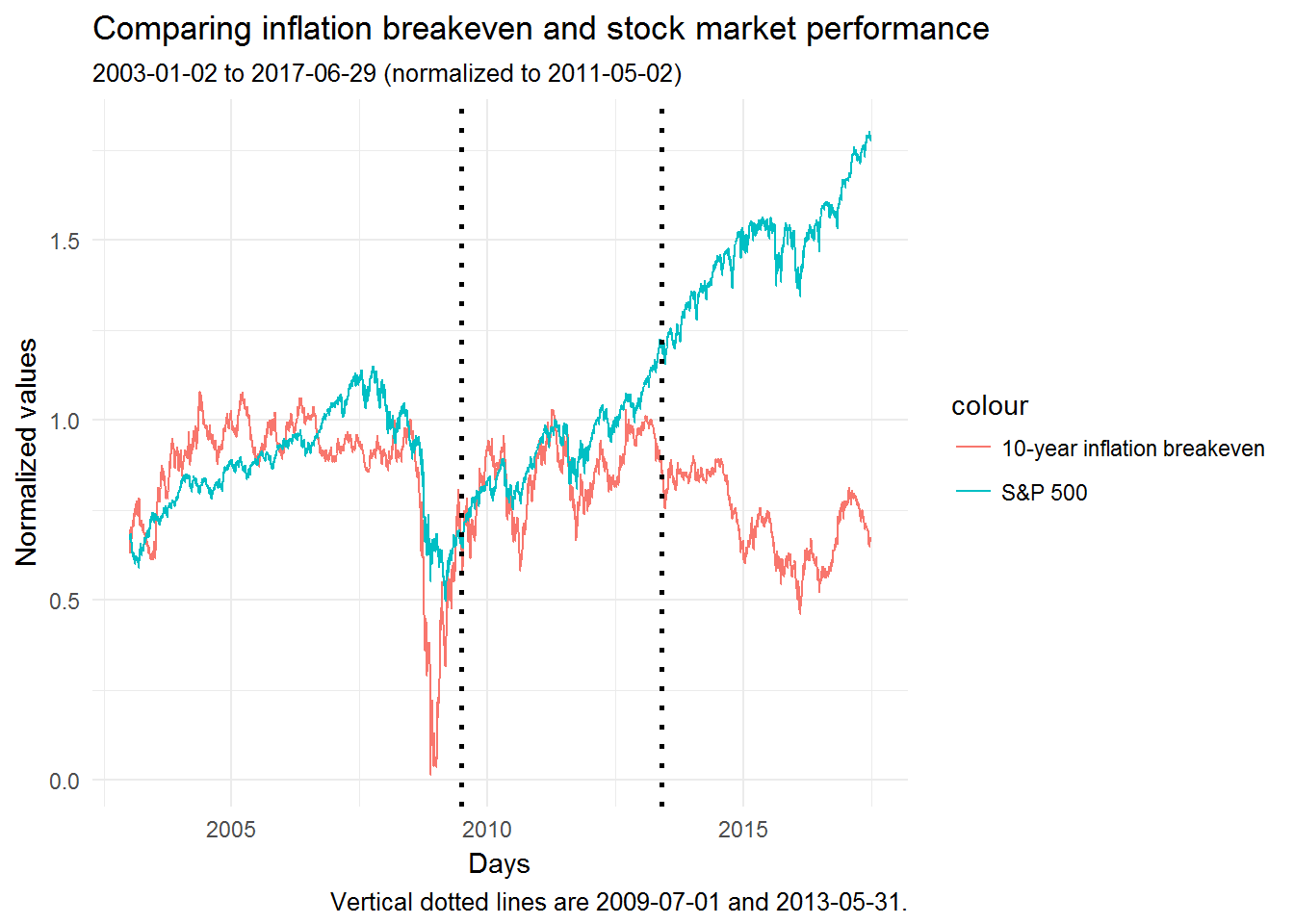
The ideal data would be \(\Delta c_{t+1}\) and \(\pi_{t+1}\) from which we could ex post calculate their correlations before and after 2008. Consumption is difficult to measure, so the authors take stock prices instead. These are claims to firms profits and as such to a piece of the aggregate cake. If the savings rate and the profit share of output don’t change too much, then taking stocks (the S&P 500 here) as a proxy for consumption growth might be reasonable.
In principle, we could just use monthly realized inflation for \(\pi_{t+1}\). But due to the short time period, the author’s take the breakeven rate (the difference between the nominal and real 10-year treasury bond yield) as a proxy for inflation expectations.2
The authors focus on the sample between the two black dotted lines. In that period, inflation expectations and the stock market were firmly positively correlated (ρ = 0.47 ± 0.028).
The story becomes very different after 2013. I wonder why that may be. The Fed Funds Rate was only raised for the first time since the crisis in December 2015. So something else seems to have been driving stocks up and inflation down in the last four years.
References
Coibion, O., Y. Gorodnichenko and D. Koustas (2017). “Consumption Inequality and the Frequency of Purchases”. NBER Working Paper No. 23357.
Fama, E. F. and G. W. Schwert (1977). “Asset returns and inflation”. Journal of Financial Economics, 5(2): 115-146.
Ngo, P and F. Gourio (2016). “Risk Premia at the ZLB: a Macroeconomic Interpretation”. Unpublished manuscript.
Somewhat counterintuitively, the breakeven rate also depends negatively on the variance of inflation. The authors explain how this “Jensen adjustment” comes about. I’m still a bit puzzled, because if “higher uncertainty about inflation leads to higher expected payoffs [for the nominal bond]” (p.6), then I’d expect the opposite sign. Maybe the effect is again through precautionary savings. The authors also write: “This term is typically small.” (p.6) ↩
That makes the argument strangely circular: We derived formula for the breakeven rate to inform us how \(\rho_t\) matters for the breakeven rate. And now we take the breakeven rate as a proxy for \(\pi_t\). But we’ve just argued that the breakeven rate is not a perfect proxy for inflation expectations, so I don’t quite see how we can do this here. ↩
A good rule of thumb is that you will want to read any working paper Melissa Dell puts out. Her main interest is the long-run path-dependent effect of historical institutions, with rigorous quantitative investigation of the subtle conditionality of the past.
Every idea taken from elsewhere can be both an asset to the development of a country and a reminder of its comparative backwardness–that is, both a model to be emulated and a threat to its national identity. What appears desirable from the standpoint of progress often appears dangerous to national independence.
In a recent paper (pdf), Olivier Coibion, Yuriy Gorodnichenko and Dmitri Koustas argue that how often we shop matters for measuring consumption inequality.
Inequality is in the focus of researchers at the moment. But usually researchers focus on inequality in income or wealth. But people probably care more about consumption than their income, so it would be good to know how consumption inequality has evolved.1 That, however, is more difficult to measure. While for income and wealth researchers can rely on some tax data, administrative data or plausible self-reported numbers, it’s hard to keep track of a person’s consumption.
The two common ways of measuring people’s consumption are (1) monthly interviews and (2) daily diaries. Consumption inequality as measured by (1) has not risen, but has increased strongly as measured by (2).
The authors’ idea of why shopping frequency matters is straightforward: The problem is that consumption is not the same as expenditures, as some goods are more durable than others. Expenditures are what we can measure and consumption is unobserved.
Some products (like toilet paper) we only buy infrequently and in bulk. So a dataset on daily toilet paper expenditures would have zeros for most people and ones for a few. So at any point in time it would look as if some people consume very much toilet paper and others none and this would imply very unequal consumption. We spend on items like food and coffee more frequently, so buying and consumption happen at times not far apart.
The authors show that people in the U.S. shop less often than they used to and argue that when you adjust for this fact, then consumption inequality has remained flat. They conclude that measuring expenditures over much longer timespans (so not days but months or quarters) is important.
Coibion et al. attribute the reduced frequency of purchases to the rise of club/warehouse stores (e.g. Wallmart). They also discuss other possible reasons for why people shop less: If people earn higher wages, then the opportunity costs of shopping might have increased. Also, houses are larger now and fridges and freezers have higher quality, so the cost of storage might have decreased.
With more online shopping, people might start buying things much more frequently again. The authors argue that this might reverse the existing trend in the mismeasurement of consumption inequality.
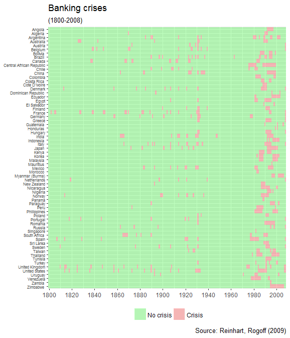
These few lines of Eric’s R code produce the following nice figure:
From this figure it becomes apparent that when banking crises happen, they tend to occur in many countries at once. We can see this happening in the early 1930s and in the 1980s and 1990s. (This sample ends in 2008.)
This observation has led some researchers (e.g. Hélène Rey) to argue for the existence of a global financial cycle.
The French philosopher Tristan Garcia wrote “La vie intense. Une obsession moderne”, which has just been published in German.
I.
The author writes that once religion offered a moral framework. But with the loss of theology, when we measure which life is worth living, we judge ourselves which means that we replaced an external morality with an internal morality. What counts is to intensely feel that we’re alive. He writes:1
Modern culture is bound to this variable intensity, a sinus curve of social electricity, a proximate measure of the collective grade of the excitement of individuals.
So we lust for a constant state of excitement and what causes the excitement is less important than the fact that we are excited:
Apparently we belong to the type of humans who have turned away from the consideration and expectation of an absolute, a transcendence as the last purpose of existence, to turn towards a certain civilization whose majority ethic depends on the unremitting fluctuation of being as its principle of life.
Garcia defines intensity as the principle of systematically comparing a thing with itself. No external rules determine its goodness or beauty. And if values are relative and there’s no objective truth, then you cannot judge a thing’s worth. You can, however, determine how extreme it is. He sounds pessimistic when he writes that we aim for the intensification of what already exists.
And because intensity is not the what, but the how, we can use ploys to spice up our bland existence. These are (1) the variation of our experiences, (2) speeding up our experiences and (3) “primaverism”, indulging in the memories of the first time we did something.
He compares the difference in the meaning of an ethic and a morality. An ethic is adverbial, it’s how you do something. A morality is adjective, it’s what you do that matters. To be ethical is to things in a good way and to be be moral is to do good things.
Garcia argues that striving for intensity was for people first a morality, but now it’s an accepted ethic:
Whether you are a fascist, revolutionary, conservative, petty bourgeois, saint, dandy, gentleman, swindler or a villain – be so energetically. Overall, it is not about being an intense person, but being intensely the person who you are. In this sense, the term succumbed to democratic change.
He explains how things that were once novel and extreme soon become standard. We get used to them, they aren’t special anymore and so we stop feeling and become emotionally numb. Near the end of the book, he invokes the image of a manic party in which people dance increasingly faster. He thinks our search for intensity can lead to fatigue and collapse.
The book’s resolution is then that we should balance rational thinking and emotional search for intensity. And we have to learn to live with the fact that the two won’t always agree.
II.
So, what does Garcia think about this? He promises to develop a morality of intensity. I thought he meant that he wants to put it into perspective, to judge it.
But we don’t find out for a long time what Garcia thinks about it, because he hides behind an impersonal voice that speaks in the present tense like the voice-over narrator in a nature documentary. Are these facts or opinions? We aren’t told. It took until page 158 that I consciously read “I” the first time. So I found his argument hard to follow because it wasn’t clear to me where those statements came from. When he invokes the reactions of people experiencing electricity for the first time, I wished Joseph Henrich would take over and explain the anthropological evidence to us.
I take his view that we’re searching intensely for what we already have to be a criticism of hedonism and complacency in our society. But I don’t see how this squares with his first ploy (aiming for more intensity through variation). If it’s novel experiences and variations that we want, then that might motivate us to innovate and come up with new or improved products and tastes.
As an economist, I’m also asking myself whether he is not just describing people being good at getting what they want. And that seems to me a good thing. Garcia himself brings up the option that we’re simply trying to feel strongly about the things we like and avoid the things we don’t. But that somehow doesn’t fit the idea of an adverbial ethic without higher meaning, so it can’t be as easy as that.
The author writes that you need a routine that you can then break out of. If everything is novel and exciting, then nothing is. The third ploy (fetishize new things) will not work forever, as there are only so many new things. That’s actually something I worry about. It seems obvious that we should try everything. Our bucket list is full things we haven’t yet done: A parachute jump or sailing across the Atlantic. Yet experiences really do become duller. When our stock of memories increases, new experiences are less thrilling.
Yet, he remains oddly silent on the benefits of intensity. Many things are cumulative and they become more intense, when you keep at them. Activitites such as playing an instrument, doing research or some types of work only become more rewarding the more you do them.
Lubos Pastor and Pietro Veronesi debate (pdf) this:
But that result [from the model in their earlier paper which says that uncertainty is bad for stocks] assumes that the precision of political signals is constant over time. In contrast, we argue here that political signals have become less precise in recent months, especially after the November 2016 election.
They state that Trump on one day says this and on another day says that. And that therefore firms get more noisy signals about the future course of economic policy and that the lack of a signal isn’t the same as uncertainty over outcomes. Their argument was also covered by the German daily FAZ(in German).
I’m not completely convinced. Maybe much of what we refer to as “economic policy uncertainty” is just firms being annoyed at regulation. Regulation, justified or not, is likely not great for corporate profits. Baker, Bloom and Davis (2016) think (especially of their industry-specific) indices as measuring “regulatory policy uncertainty” (p.1621). But what if it’s more a proxy for “regulatory policy”?
It’s like when people say “risk has gone up”, they often only refer to downside risk. With Trump, I think, actual “uncertainty” (or what Pastor and Veronesi call “the precision of political signals”) is up, but the expected value of how much regulation there will be is far down. So expected profits rise and thus stocks benefit. But at the same time the newspapers are full of the words “uncertainty”, because there really is uncertainty about the future course of regulatory policy.
I had a try at Schelling’s segregation model, as described on quant-econ.
In the model, agents are one of two types and live on (x,y) coordinates. They’re happy if at least half of their closest 10 neighbors are of the same types, else they move to a new location.
My codes are simpler than the solutions at the link, but I actually like them like this. In my codes, agents just move to a random new location if they’re not happy. In the quant-econ example they keep moving until their happy. And I just simulate this for fixed number of cycles, not until everyone is happy.
In Matlab:
n=1000;% number of agents of one typeN=2*n;% total number of agentsT=10;% number of cycleslocs=rand(N,2);% initial locationtypes=[ones(n,1);% generate two typeszeros(n,1)];figureset(gca,'FontSize',16)scatter(locs((types==1),1),locs((types==1),2))holdonscatter(locs((types==0),1),locs((types==0),2))title('Cycle 0')print('test0','-dpng')holdofffort=1:Tfori=1:N% All other agentsothers=[locs(1:(i-1),:);locs((i+1):end,:)];% Distance to other agentsdist=pdist2(locs(i,:),others)';% Nearest other agents[~,ix]=sort(dist);nearestAgents=(ix<=10);% Neighbors of same typesameNeighbors=sum(types(i)==types(nearestAgents));% Happy if at least 5 of neighbors are same typeisHappy=(sameNeighbors>=5);% If not happy, then move to random new locationifnot(isHappy)locs(i,:)=rand(1,2);endendfprintf('Finished cycle %d/%d.\n',t,T)figureset(gca,'FontSize',16)scatter(locs((types==1),1),locs((types==1),2))holdonscatter(locs((types==0),1),locs((types==0),2))title(['Cycle ',num2str(t)])print(['test',num2str(t)],'-dpng')holdoffend
Which yields the following sequence of images:
The two groups separate quickly. Most of the action takes place in the first few cycles and after the remaining minority types slowly move away into their type’s area.
In the paper, Schelling emphasizes the importance of where agents draw their boundaries:
In spatial arrangements, like a neighborhood or a hospital ward, everybody is next to somebody. A neighborhood may be 10 percent black or white; but if you have a neighbor on either side, the minimum nonzero percentage of neighbors of either opposite color is fifty. If people draw their boundaries differently, we can have everybody in a minority: at dinner, with men and women seated alternately, everyone is outnumbered two to one locally by the opposite sex but can join a three-fifths majority if he extends his horizon to the next person on either side.
We have a new working paper out with the title “Benign Effects of Automation: New Evidence from Patent Texts”. You can find it here. Any comments are much appreciated.