Term spreads and business cycles 1
The term spread is the return differential between a long-term and a short-term safe bond. We can use this to learn about how market participants expect the economy to perform over the next year or so.
My explanation loosely follows Stephen Cecchetti and Kermit Schoenholtz’s book “Money, Banking, and Financial Markets”.
I.
Consider an investor who either buys a long-run bond running for two years and pays \(i_{2,t}\) per year or he invests in two subsequent short-run bonds. If he chooses the second option, the bond pays \(i_{1,t}\) in the first year and he expects to earn \(i^e_{1,t+1}\) in the second year. If we neglect any risk, it’s plausible to assume that interests rates adjust such that the investor earns the same using either strategy:
\[(1 + i_{2,t})(1 + i_{2,t}) = (1 + i_{1,t})(1 + i^e_{1,t+1}).\]When we evaluate this expression and omit all terms that multiply two rates (these will typically be small), we get:
\[i_{2,t} = \frac{i_{1,t} + i^e_{1,t+1}}{2}\]We can extend this for any years n:
\[i_{n,t} = \frac{i_{1,t} + i^e_{1,t+1} + \dots + i^e_{1,t+n-1}}{n}\]So long-term interest rates are composed of expectations about future short term interest rates.
Combine this with what the Cecchetti and Schoenholtz call the Liquidity Premium Theory. Returns that accrue farther into the future are more risky, as the bond issuer may be bankrupt and we don’t know what inflation will be. This means that rates on bonds with longer maturities are usually higher.
The authors add a factor \(rp_n\) (the risk premium of a bond running \(n\) years) to the original equation:
\[i_{n,t} = rp_n + \frac{i_{1,t} + i^e_{1,t+1} + \dots + i^e_{1,t+n-1}}{n}\]As \(rp_n\) is higher for greater \(n\), interest rates will tend to be higher for longer maturities.
The term spread \(ts_{n,t}\) is then
\[\begin{align} ts_{n,t} &= i_{n,t} - i_{1,t} \nonumber \\ &= rp_n - rp_1 + \frac{i_{1,t} + i^e_{1,t+1} + \dots + i^e_{1,t+n-1}}{n} + i_{1,t} \label{term_spreads} \end{align}\]A positive term spread can mean two things. Either we expect the average future short-term interest rate to rise or the difference between the two risk premia (\(rp_n - rp_1\)) has increased. We would expect this difference to be positive anyway, but it might widen even more when inflation becomes more uncertain or debt becomes riskier. But disentangling the two explanations is difficult.
It’s more interesting when the term spread turns negative. The difference between the risk premia probably stays positive, so investors expect short-term interest rates to decrease.
Short-term interest rates are mostly under the control of the central bank, so this probably means that people expect monetary policy to loosen and that the central bank lends more liberally to banks.
And why would the central bank do that? That’s usually to avert a looming recession and buffer negative shocks. Given that the central bank also responds to changes in the economic environment, it’s not clear what’s causing what here.
But either way, when term spreads turn negative, investors expect bad things. This is why the term spread tells us something about investors’ expectations.
II.
Let’s look at the empirical evidence for this, as argued and presented by the authors. They kindly provide Fred codes with all their plots, so they’re easy to reproduce. First get some packages in R:
library(tidyverse)
install.packages("devtools")
devtools::install_github("jcizel/FredR")
library(zoo)
library(lubridate)
library(ggthemes)
Insert your FRED API key below:
api_key <- "yourkeyhere"
fred    <- FredR(api_key)
Pull data on 10 year and 3 month treasury bill rates:
# Long-term interest rates
fd <- fred$series.observations(series_id = "GS10") %>%
  mutate(date = as.Date(date)) %>%
  select(date, t10 = value) %>%
  mutate(t10 = as.numeric(t10))

# Short-term interest rates
fd <- fred$series.observations(series_id = "TB3MS") %>%
  mutate(date = as.Date(date)) %>%
  select(date, tb3m = value) %>%
  mutate(tb3m = as.numeric(tb3m)) %>%
  full_join(fd)

# Turn dates into month-years and order by dates
fd <- fd %>%
  mutate(date = as.yearmon(date)) %>%
  arrange(date)
Plot the two series:
fd %>%
  gather(var, val, -date) %>%
  ggplot(aes(date, val, color = var)) +
  geom_hline(yintercept = 0, size = 0.3, color = "grey80") +
  geom_line() +
  labs(title = "The Term Structure of Treasury Interest Rates",
       subtitle = "1934-2017, monthly",
       x = "month",
       y = "yield",
       color = "Treasury bill:") +
  scale_color_manual(labels = c("10-year", "3-month"),
                     values = c("#ef8a62", "#67a9cf"))  +
  theme_tufte(base_family = "Helvetica")
Which produces:
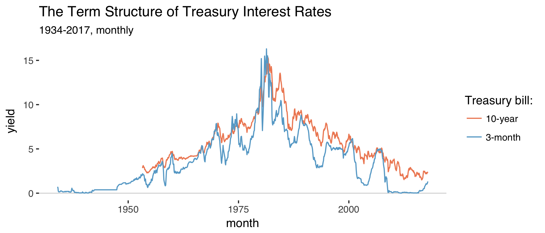
The series on 3-month Treasury bond yields starts in 1934 and the other series on 10-year yields starts in 1953. Both series peak in the early 80s when inflation ran high. As argued before, long-run interest rates are usually above short-run interest rates. The term spread is the difference between the two:
fd <- fd %>%
  mutate(trm_spr = t10 - tb3m)
Things become more interesting when we compare the behavior of the term spread with real GDP growth rates:
# Get quarterly GDP
qt <- fred$series.observations(series_id = "GDPC1") %>%
  mutate(yq = as.yearqtr(paste0(year(date), " Q", quarter(date)))) %>%
  select(yq, rgdp = value) %>%
  mutate(rgdp = as.numeric(rgdp),
         gr = 100*(rgdp - dplyr::lag(rgdp, 4)) / dplyr::lag(rgdp, 4))

# Aggregate monthly to quarterly and get lag
qt <- fd %>%
  mutate(yq = as.yearqtr(date)) %>%
  group_by(yq) %>%
  summarize(trm_spr = mean(trm_spr)) %>%
  mutate(trm_spr_l = dplyr::lag(trm_spr, 4)) %>%
  full_join(qt, by = "yq") %>%
  filter(yq >= "1947 Q1")
Make a plot of the two series:
qt %>%
  select(-rgdp, -trm_spr_l) %>%
  drop_na(trm_spr) %>%
  gather(var, val, -yq) %>%
  ggplot(aes(yq, val, color = var)) +
  geom_hline(yintercept = 0, size = 0.3, color = "grey80") +
  geom_line() +
  labs(title = "Current Term Spread and GDP Growth",
       subtitle = "1953-2017, quarterly",
       x = "quarter",
       y = "percentage points",
       color = "Variables:") +
  theme_tufte(base_family = "Helvetica") +
  scale_color_manual(labels = c("Real GDP growth", "Term spreads (lagged)"),
                     values = c("#ef8a62", "#67a9cf"))
We get:
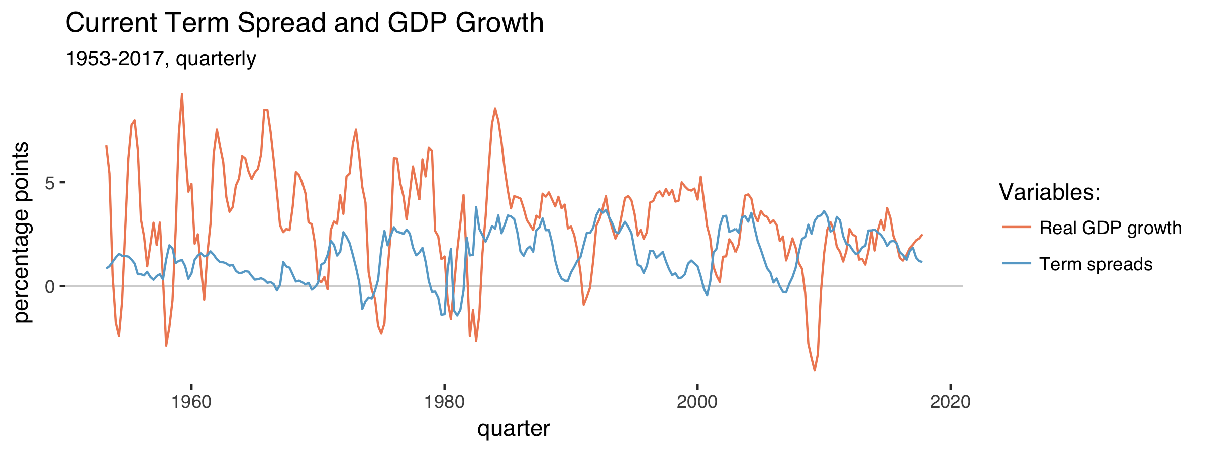
The term spread often falls before GDP growth does. When the term spread turns negative, recessions tend to happen. Compare the lagged term spread to GDP growth:
qt %>%
  filter(yq >= 1953) %>%
  ggplot(aes(gr, trm_spr_l)) +
  geom_hline(yintercept = 0, size = 0.3, color = "grey50") +
  geom_vline(xintercept = 0, size = 0.3, color = "grey50") +
  geom_point(alpha = 0.7, stroke = 0, size = 3) +
  labs(title = "Term Spread 1 Year Earlier and GDP Growth",
       subtitle = paste0("1953-2017, quarterly. Correlation: ",
                         round(cor(qt$gr, qt$trm_spr_l,
                                   use = "complete.obs"), 2), "."),
       x = "growth rate of real GDP",
       y = "Term spread (lagged 1 year)") +
  geom_smooth(method = "lm", size = 0.2, color = "#ef8a62", fill = "#fddbc7") +
  theme_tufte(base_family = "Helvetica")
Which gets us:
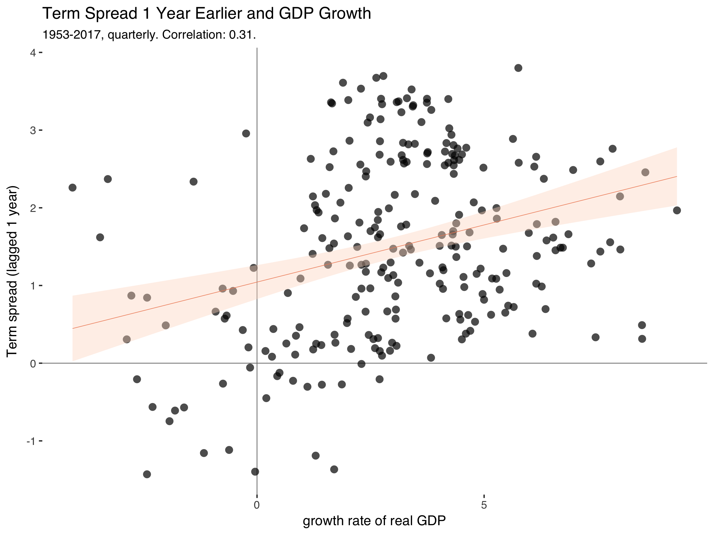
This is exactly the relationship that makes people think of term spreads as a good predictor of GDP in the near future.
III.
Cecchetti and Schoenholz summarize it like this (p.180):
[…] [I]nformation on the term structure – particularly the slope of the yield curve – helps us to forecast general economic conditions. Recall that according to the expectations hypothesis, long-term interest rates contain information about expected future short-term interest rates. And according to the liquidity premium theory, the yield curve usually slopes upward. The key statement is usually. On rare occasions, short-term interest rates exceed long-term yields. When they do, the term stucture is said to be inverted, and the yield curve slopes downward.
[…] Because the yield curve slopes upward even when short-term yields are expected to remain constant – it’s the average of expected future short-term interest rates plus a risk premium – an inverted yield curve signals an expected fall in short-term interest rates. […] When the yield curve slopes downward, it indicates that [monetary] policy is tight because policymakers are attempting to slow economic growth and inflation.
We still don’t know what’s causing what. Is the central bank the driver of business cycles or is it just responding to a change in the economic environment?
Stay tuned for the next installment in this series in which I’ll look at the role of monetary policy.
References
Cecchetti, S. G. and K. L. Schoenholtz (2017). “Money, Banking, and Financial Markets”. 5th edition, McGraw-Hill Education. (link)